Jo Kondo’s
Still Life
Appendix
App. i
Distributions of and within “agg”s.
Ex. 19 sorts all “agg”s by the number of different “P”s per “agg”. Colored symbols above some “agg”s are explained later in the main text. Meas. numbers appear beneath “agg”s. “Aggs” that repeat show multiple meas. numbers.
The following table summarizes the sort:
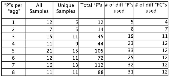
where the first col. tells how many “P”s per “agg” category (1 - 8); the 2nd col. tells how many “agg”s are of the specific type (i.e. the composition has a total 12 “agg”s that contain one “P”); the 3rd col. tells how many of these “agg”s are different (i.e. there are 5 unique samples of “P” = 1, and some of these repeat, for a total of 12 “agg”s containing one “P”); the 4th col. tells the total number of “P”s (i.e. found by multiplying cols 1 & 2); and the last two cols. tell the number of different “P”s and “PC”s utilized (“agg”s containing one “P” use 5 different “P”s, but as the C natural appears in two different octaves, “agg”s containing one “P” use a total of 4 “PC”s).
This ex. helps bring registral divisions to the fore i.e. consider “agg” size 8, where “P”s are sometimes almost uniformly distributed across registers (meas. 9 or 31); vs. a more bifurcated distribution (meas. 34 with (from the bottom up) 2 “P”s + 6 “P”s; or meas.s 36 & 99 with two groups of 4 “P”s; vs. meas. 81 (2 + 4 + 2); etc.). As such distribution differences exist for all “agg” sizes, “agg”s could perhaps be sorted (across size categories) based upon these different registral distributions.
One might wish to use Ex. 19 to trace the accretion of "agg"s (from 1 to 2 to 3 etc “P”s), but it is difficult to do so. This may be due (somewhat) to variances in the distributions of "P" as a function of "agg" size, and for that, we turn to Ex. 20, which sorts “P”s by frequency of use per “agg” size.
This matrix (using the total number of times a specific “P” is played by all violinists (see Ex. 3) is read as follows. Columns represent “agg” sizes. “P”s appear in rows ranked by frequency of use (i.e. for “agg” size 1, “P” = “D4” is played by 33 violinists; “A3” is played by 16; etc.; the fewer the violins playing, the lighter the red background). Note how the most frequent “P”s of the top 5 rows vary across col.s as “agg” size increases. REMEMBER: col.s are not slices of time, i.e. reading across col.s is NOT reading thru the composition. Col.s are only “agg” sizes, no matter where (in the composition) the “agg” occurs. This matrix says that different “agg” sizes, each taken as a group, may differ (substantially) in terms of their palettes of “P”s, and their internal emphases. This point is even more manifest when we observe the differences in the number of “P”s used per "agg", where “agg” sizes 5, 7 and 8 use 31-33 "P"s; as opposed to "agg" sizes 3, 4 and 6 with far fewer "P"s. Such differences can NOT be solely attributed to arithmetic i.e. the number of “total” “P”s used for each different “agg” size can not fully explain the number of “different” “P”s employed for that “agg” size. Sample sizes are far too small for any of the counts (let alone their interactions) in this text to rise to statistical significance; but this hint of how “P” and/or “PC” prominence differs between, and how the palette of “P” and/or “PC” perhaps depends upon, “agg” size, may prove worthy of further study in other Kondo compositions.
Much has been made (with more to come) of “PC” vs. “P”. To help simplify this sometimes opaque aspect, ex. 21 presents the composition as a spreadsheet of “PC”s, condensed from an original specifying all “P”s. We hasten to stipulate that normally composers do not write using “PC”s, and especially for Kondo, a specific “P” far outweighs its “PC” counterpart. Nevertheless, thinking in terms of “PC”s allows one to more simply classify certain aspects and relationships of the “aggs”, relationships that otherwise might go unnoticed. In ex. 21, time is horizontal i.e. col.s represent meas. (numbered at the top, with the 10 meas. per “line” of music being maintained). Pitch is vertical, with “PC”s listed at the left. Numbers within a spreadsheet-cell tell the number of violinists playing the specific “PC”. Red and blue horizontals correspond to the horizontals of ex. 9 (i.e. lengths of 5 meas. or greater). Clusters are hatched, as detailed at the bottom right. Triads labels, corresponding to ex. 11 etc., are highlighted in purple. A summary of “PC”s, “P”s, no. of clusters and types, appears below the triads.
There are advantages viewing the work in this format. First, the specifics of the “PC” clusters are easier to see and compare. Next, there is greater clarity in regards how clusters may act as “attractants”, and may progress over time (just as triads can wiggle about from “harmonic” area to area (think Reger “Theory of Modulation”?), so too can clusters). As example, on page one, the C/C#/D triune moves (in meas. 5) to F#/G/G#; then an additional 1/2- step shift to G/G#/A; then a “slip” downwards (in “PC” terms, not visually!) to E/F/F#. Similar wanders occur thruout the work, and are analogous to triad wanders (i.e. a passage such as meas. 56 - 71 from F to f# to G to C (with digressions)).
This matrix also provides perspectives different from those of the exs. in the main body. There, horizontal supremacy is emphasized, followed by triads; with dyads, triunes and ovals as a tertiary matter. Ex. 21 shows that hatches, together as a single group, permeate the landscape more than previously indicated. The numbers are:
68 meas. contain hatches; of which
26 are without triads; 42 are with triads.
51 meas. contain triads; of which
9 are without hatches; 42 are with hatches.
i.e., meas. with hatches account for 64.8% of the total 105 meas.; and a more representative hierarchy might be horizontals (at 72 meas. -- see ex. 8), followed by hatches, followed by triads. Also note how matrix pages (aka lines of music) vary -- some with few triads; some with few hatches; hatches sometimes primary; triads sometimes primary; some pages rather bare, others quite quite murky; and the matrix may shed light on the interplay, intertwine, and interaction of horizontals and verticals. For insight beyond the scope of this data-driven text, look beyond “music” (Klee’s “Pedagogical Sketchbook”, or “Notebooks”, come to mind). As a further advantage, “flipping” thru the pages (as if in a flip-book) helps one to see the overall progression without getting lost amongst the individual trees.
App. ii
All about “agg”-pairs
Plotting “agg”-pairs on a grid of 5 rows x 21 cols. (ex. 22) reveals a pair - letter at the midpoint of each 21-measure span – i.e. the pink swath with the letters “D”, “H”, “K”, “M” and “D” (“D”/”D” being one of only three pairs that repeat in the same column, the others being “C”/”C” and “G”/”G”). Note the skewed distribution, i.e. far more pairs appear to the right of the pink swath, than to the left.
Adding “agg”s that repeat more than twice (ex. 23) shows an even greater concentration of repeated “agg”s to the right of the pink swath, with “agg”s appearing only once (i.e. the empty meas.) concentrated to the left of the swath. The red-colored “agg”s of meas. 15, 38, 61, 76 and 101 all appear to the right of the midline swath. Note that other plots of aliquot factors of 105 (3 X 35; 7 X 15) do not show even this much pattern, and the pink swaths of ex.s 18, 22 and 23 may simply be a matter of apophenia, without musical function.